The Data Menu
The Data menu provides access to global libraries and settings that affect the underlying physics and economics of your simulation. Instead of configuring these values on every individual component, you define them here once and reference them throughout your project.
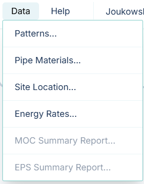
Here is a breakdown of every option in the Data menu:
Patterns...
Opens the Manage Patterns dialog. Patterns are time-variable multipliers used to represent changes over a 24-hour period (such as fluctuating water demands or time-of-use energy rates).
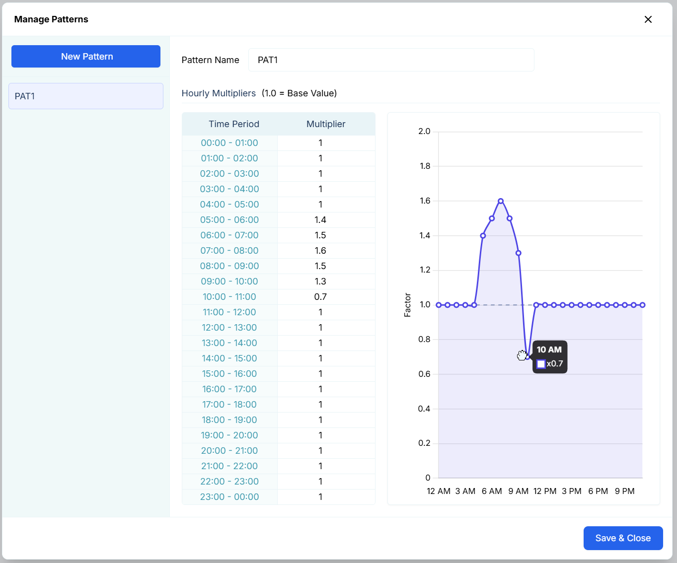
[!TIP] While you can type exact multipliers into the table, you can also graphically adjust the pattern by simply clicking and dragging the points on the chart with your mouse! We will discuss how to apply these patterns to specific components later in the manual.
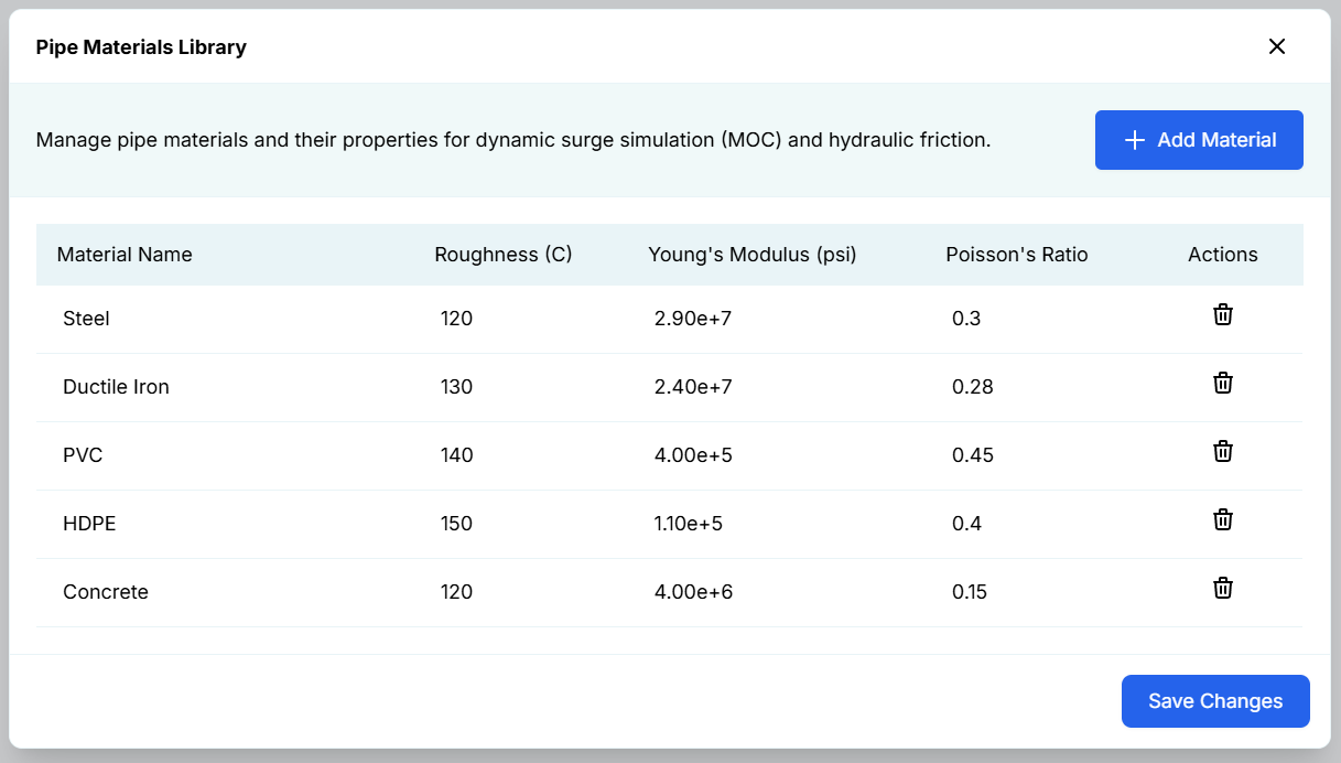
Pipe Materials...
Opens the Pipe Materials Library. Here, you define the physical properties of various pipe materials (such as Roughness (C), Young's Modulus, and Poisson's Ratio). These properties are utilized across both simulation modes: the Roughness (C) coefficient is used for standard EPS friction calculations, while Young's Modulus and Poisson's Ratio are critical for calculating wave speed during dynamic transient (MOC) simulations.
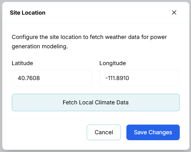
Site Location...
Opens the Site Location configuration. By entering the Latitude and Longitude of your project site, R-THYM can fetch local climate data (including sunrise/sunset times, ambient temperature, solar radiation, and wind speed). This environmental data is directly utilized by the Solar and Wind power generation components to accurately model renewable energy yields.
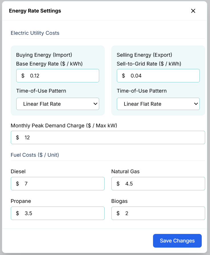
Energy Rates...
Opens the Energy Rate Settings dialog, which calculates the economic impact of your system. This dialog is highly versatile:
- Buying/Selling Power: Define the base rates for importing power to run pumps, or exporting (selling) power back to the grid from Hydropower, Wind, and Solar generators.
- Time-of-Use Pattern: You can link the rates to the Patterns discussed above to simulate complex, time-variable pricing.
- Peak Demand Charges: Set a charge applied to your maximum kW peak (note that peak demand often occurs during pump startup when it must push hardest against the static head).
- Fuel Costs: Define the unit cost of Diesel, Natural Gas, Propane, and Biogas for your backup generators.
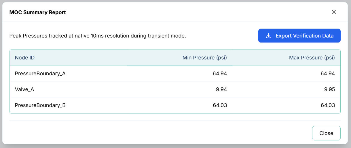
MOC & EPS Summary Reports...
These options generate comprehensive summary screens of your static (EPS) or transient (MOC) runs and provide a button to export the data as a .zip archive.
When you export EPS Data, the zip file contains:
R-THYM_EPS_Summary.json: Contains your project settings, total simulated hours, warning logs, and aggregated economic metrics like total energy costs, total water delivered, fuel consumed, and the system's min/max pressures.R-THYM_EPS_Traces.csv: A time-series log of your simulation. To keep file sizes manageable, it dynamically strides the data to a maximum of 10,000 rows. It automatically creates columns based on the components in your model, tracking attributes like Tank Levels, Pump Flows/Power, Junction Pressures, Pipe Velocities, and environmental variables (Temperature/Wind/Solar).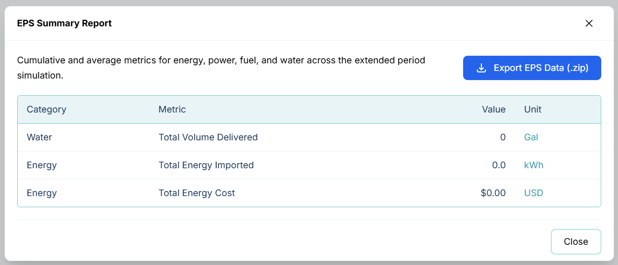
When you export MOC Verification Data, the zip file contains:
R-THYM_MOC_Verification.json: Contains transient-specific metadata, including control rules and explicitly generated valve closure schedules (identifying the exact start and end seconds of a surge event).R-THYM_MOC_Traces.csv: A high-resolution time-series log tracking the pressure (psi) and flow (gpm) for your nodes during the transient event. This is recorded at the native 10ms engine resolution to accurately capture rapid water hammer spikes.