Utility Grid
The Utility Grid component serves as your infinite source and sink for electrical power. It represents your connection to the local electrical distribution system (such as a local municipal utility or regional provider).
Unlike traditional modeling software that may treat energy costs as a secondary calculation based entirely on pump runtime, R-THYM explicitly maps electrical paths using Power Links. To power a pump or charge a battery, you must connect a path from the Utility Grid (or another power source) to the load.
UI Workflow and Configuration
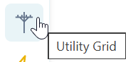
To add a Utility Grid to your model, click the Utility Grid icon (which resembles a power transmission pole) in the Component Toolbar and drag it onto the canvas.
You can configure its properties by double-clicking the icon or right-clicking and selecting Properties.
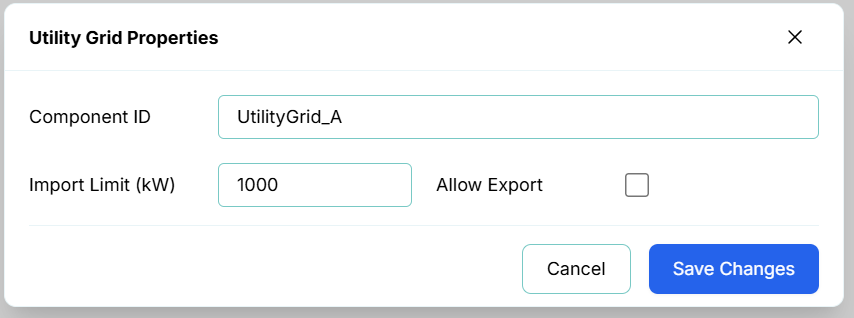
The properties dialog focuses on the core parameters that drive the physical engine and energy tracking:
- Component ID: A unique string identifier for the grid connection (e.g.,
Grid_Main). - Import Limit (kW): The maximum capacity of the grid connection (i.e., your main breaker or transformer size). If your downstream pumps or batteries attempt to draw more power than this limit allows, the power simulation will bottleneck, and downstream equipment will fail to start or will run at reduced capacity due to power starvation.
- Allow Export: A toggle that permits excess renewable energy (e.g., from Solar Generators or Turbines) to flow backwards through the grid connection for revenue.
[!NOTE] Why is "Allow Export" a toggle? In the real world, many electrical utilities do not allow net metering, or they require special interconnection agreements before you can export power back to the grid. If you connect solar but are not permitted to export, the system will automatically curtail solar production once your batteries are 100% full. Having this toggle allows you to accurately model both scenarios.
Energy Rates
Connecting your equipment to the Utility Grid inherently ties their energy consumption to the Energy Rate Settings defined in the Data Menu.
Applying a Time-of-Use Pattern
To configure time-varying financial costs for this power:
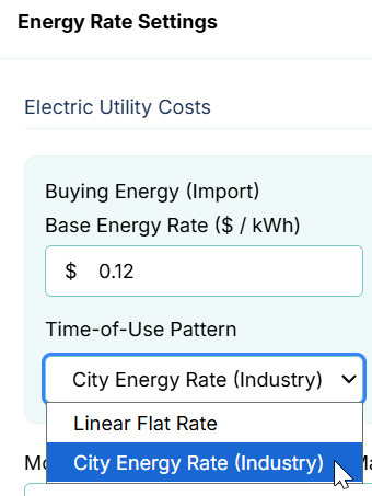
- Navigate to Data -> Patterns... in the top menu bar to create a new diurnal multiplier pattern (e.g., "City Energy Rate (Industry)").
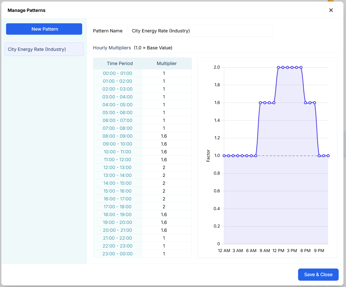
- Navigate to Data -> Energy Rates... to open the utility cost settings.
- Under the "Buying Energy (Import)" or "Selling Energy (Export)" sections, click the Time-of-Use Pattern drop list selector and choose the pattern you just created.
Peak Demand Charges
Many industrial power consumers are billed not just for the total energy they consume (kWh), but for the maximum rate at which they consumed it (Peak kW).
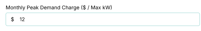
By setting a Monthly Peak Demand Charge ($ / Max kW) in the Energy Rates dialog, R-THYM will continuously monitor the maximum power drawn through the Utility Grid during the simulation. This peak value is multiplied by the Demand Charge rate to calculate an estimated demand penalty, which is directly factored into the overall operational cost.
Live Telemetry
Left-clicking a Utility Grid on the canvas reveals its performance data and financial metrics in the right-hand Telemetry Panel.

The panel tracks:
- Instantaneous Power: The real-time Grid Flow (kW) showing whether you are currently importing or exporting power.
- Energy Tracking: Cumulative Energy (Import) and Energy (Export) measured in kWh.
- Financial Metrics: The real-time accumulated Import Cost based on your Base Rate and Time-of-Use multiplier, as well as the Est. Demand Charge calculated from the recorded Peak Demand (kW).
- Dynamic Charts: Visualizes the Power Flow alongside the cumulative Energy and tracked Costs/Revenues over the duration of the simulation.
[!TIP] System-Wide Telemetry While the Utility Grid panel shows the metrics for that specific grid connection, you can click on an empty space on the canvas to view the System Overview telemetry. The System Overview aggregates the total power, total energy, and total operational cost across the entire digital twin, providing a comprehensive financial summary of your modeled scenario.
