PID Control Links
While deadband controllers handle binary ON/OFF states, many modern hydraulic and energy systems require continuous adjustment. Variable Frequency Drive (VFD) pumps must speed up or slow down to maintain a constant pressure, and modulating valves must adjust their opening percentages to regulate flow.
R-THYM supports continuous feedback control using the Proportional-Integral-Derivative (PID) control algorithm.
How PID Works in R-THYM
A PID controller continuously monitors the difference between a desired Target Setpoint ($r(t)$) and a measured Monitored Parameter ($y(t)$). This difference is the control error ($e(t)$):
$$e(t) = r(t) - y(t)$$The controller calculates its output $u(t)$ using a combination of three terms:
$$u(t) = K_p e(t) + K_i \int_0^t e(\tau) d\tau + K_d \frac{de(t)}{dt}$$Where: * $K_p$ is the Proportional Gain * $K_i$ is the Integral Gain * $K_d$ is the Derivative Gain
For example, the pump speed factor ($0.0 \text{ to } 1.0$) or the valve opening ratio ($0\% \text{ to } 100\%$).
Discrete-Time Simulation
Because R-THYM runs a discrete-time dynamic simulation with a time step of $\Delta t$, the continuous equations are converted into discrete form for each simulation tick $n$:
$$u_n = K_p e_n + K_i \sum_{j=0}^{n} (e_j \Delta t) + K_d \frac{e_n - e_{n-1}}{\Delta t}$$The Three Terms Explained
To set up a stable simulation, it is essential to understand how each parameter influences your hydraulic network:
1. Proportional ($K_p$)
Reacts to the current error. If the monitored pressure is far below the target, the proportional term outputs a large correction to speed up the pump or open the valve.
- Limitation: A proportional-only ($P$) controller can never eliminate the error completely. It always exhibits a steady-state offset. As the error approaches zero, the controller output also approaches zero, meaning the pump slows down before the target is fully met.
2. Integral ($K_i$)
Reacts to the accumulated history of the error. If a steady-state offset persists over time, the integral term continues to add up the error, steadily increasing the control output until the monitored value reaches the target.
- Limitation: While the integral term eliminates the steady-state offset, it can cause the system to overshoot or oscillate if configured too aggressively.
3. Derivative ($K_d$)
Reacts to the rate of change of the error, acting as a brake. If the monitored variable is rapidly approaching the target, the derivative term subtracts from the control output to prevent overshooting.
- Limitation: In hydraulic simulations, flow rates and pressures can change abruptly due to other network events. A high $K_d$ can amplify these sudden changes, leading to solver instability.
UI Configuration
To configure a PID Control Link:
- Double-click the Control Link (or right-click it and select Properties).
- Set the Strategy to
PID (Variable Speed/Position). - Configure the following properties in the dialog:
| Property | Description | Typical Ranges / Examples |
|---|---|---|
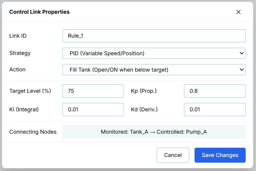
| Link ID | The unique identifier for this control link rule (e.g., Rule_1). |
— |
| Strategy | The control scheme to apply. Select PID (Variable Speed/Position). |
— |
| Action | The operation behavior defining how the controller reacts to the setpoint (e.g., Fill Tank (Open/ON when below target)). |
— |
| Target Level (%) | The target level percentage the controller aims to maintain (e.g., 50%). |
0 to 100% |
| Kp (Prop.) | Proportional Gain ($K_p$) — multiplier for the immediate error. | 0.1 to 2.0 (e.g., 0.7) |
| Ki (Integral) | Integral Gain ($K_i$) — multiplier for the accumulated error. | 0.01 to 0.5 (e.g., 0.05) |
| Kd (Deriv.) | Derivative Gain ($K_d$) — multiplier for the rate of change of error. | 0.0 to 0.1 (e.g., 0.02) |
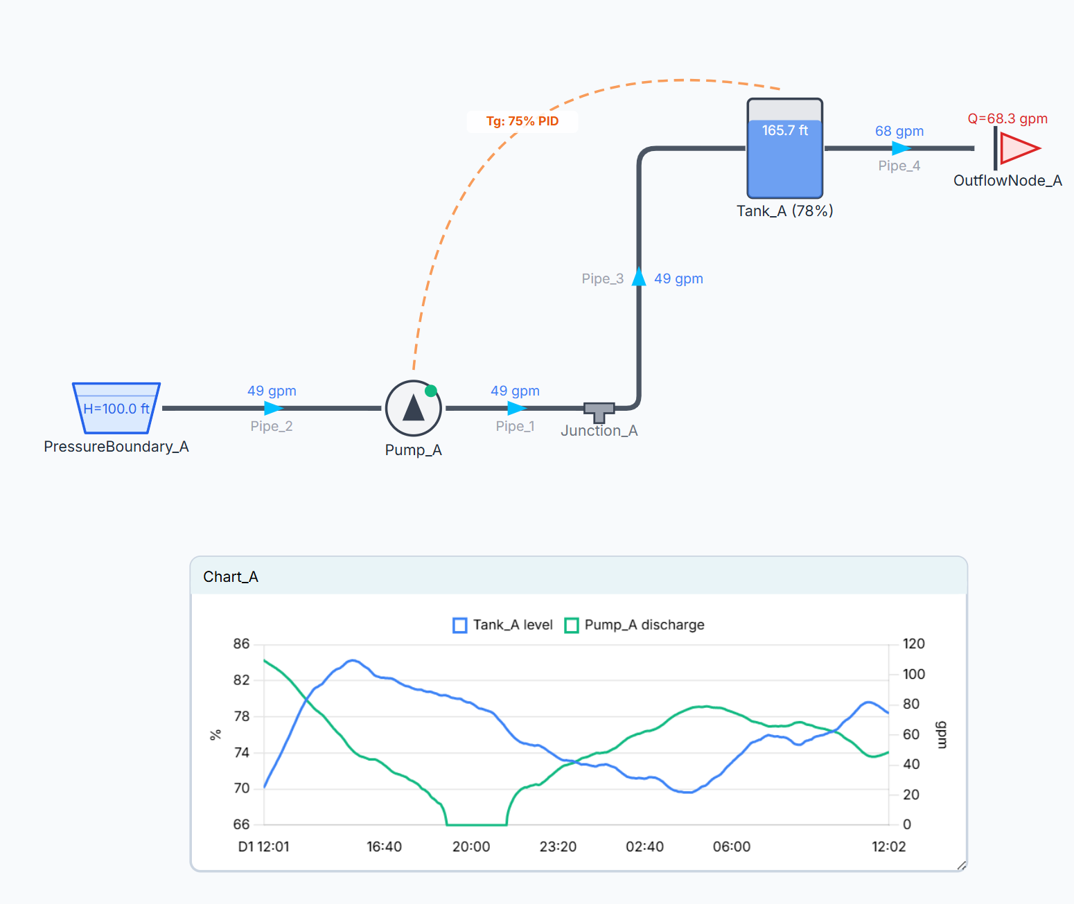
| Connecting Nodes | A read-only field displaying the monitored source node and the controlled target element. | e.g., Monitored: Tank_A → Controlled: Pump_A |
Integral Windup and Anti-Windup Clamping
A common issue in physical and simulated controllers is Integral Windup. If a pump is sized to deliver a maximum of 50 psi, but the user configures the target setpoint to 80 psi: 1. The error $e(t)$ will remain positive. 2. The integral term will continuously accumulate this error, winding the output value up to a massive number (e.g., $u_n = 5000\%$). 3. If the downstream demand suddenly drops and the pressure rises, the controller will not slow the pump down immediately. It must first wait for the accumulated integral error to slowly wind down, leading to massive overpressure and surge behavior.
R-THYM prevents this by implementing Anti-Windup Clamping: If the computed controller output $u_n$ reaches either Output Min Limit or Output Max Limit, the accumulation of the integral term is temporarily paused (clamped) until the sign of the error reverses. This ensures the digital twin behaves stably during extreme operating conditions.
Modeling Best Practices: Tuning PID in R-THYM
Tuning a PID controller in a hydraulic network is different from tuning one in a mechanical or thermal system because hydraulic responses are nearly instantaneous. Use this systematic approach:
- Start with Proportional-Only ($K_p$): Set $K_i = 0$ and $K_d = 0$. Run the simulation and increase $K_p$ until the monitored parameter approaches the target setpoint quickly. If you see the pump speed or valve position oscillating rapidly between time steps, decrease $K_p$.
- Add Integral ($K_i$) to Remove Offset: You will notice that under $P$-only control, the monitored value stabilizes slightly below your target (the offset). Slowly increase $K_i$ (start with small increments like
0.05) until this offset is eliminated over a few simulation steps. - Leave Derivative ($K_d$) at $0$: In almost all hydraulic digital twins, $K_d$ should remain
0.0. The instantaneous nature of hydraulic calculations in network solvers means that derivative control often introduces noise and numerical instability without providing any real-world benefit.