Outflow Node
The Outflow Node (often referred to as a "Demand Node" in standard EPANET terminology) is the primary method for modeling water leaving your hydraulic system. It represents consumer usage, industrial processes, agricultural irrigation, or any other localized draw.
While a standard Junction can theoretically have a negative inflow to represent demand, the Outflow Node in R-THYM is specifically designed with advanced tools for modeling time-varying and stochastic demands during Extended Period Simulations (EPS).
UI Workflow and Configuration
To add an Outflow Node, select its icon from the Component Toolbar and drag it onto the canvas.

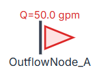
Notice that the node displays its real-time draw (e.g., Q=50.0 gpm) directly above the icon during active simulations.
Double-click or right-click the node and select Properties to configure it.

The core physical properties include:
- Base Demand (gpm): The nominal, steady-state flow rate expected to leave the system at this location.
- Elevation (ft): Crucial for calculating the local delivery pressure.
- Min Pressure (psi): Sets a service threshold to trigger telemetry warnings if the pressure drops below acceptable limits (e.g., 5 psi) due to excessive draw or pipe failures.
Flow Rate Patterns (Diurnal Curves)
In reality, water demand is rarely constant. To accurately model an EPS run over multiple days, you need to apply a Pattern to the Base Demand.

Selecting a pattern (like "Irrigation Demand") applies a time-varying multiplier to the Base Demand. To create or edit patterns, open the Manage Patterns dialog (accessible via the main toolbar or project settings).
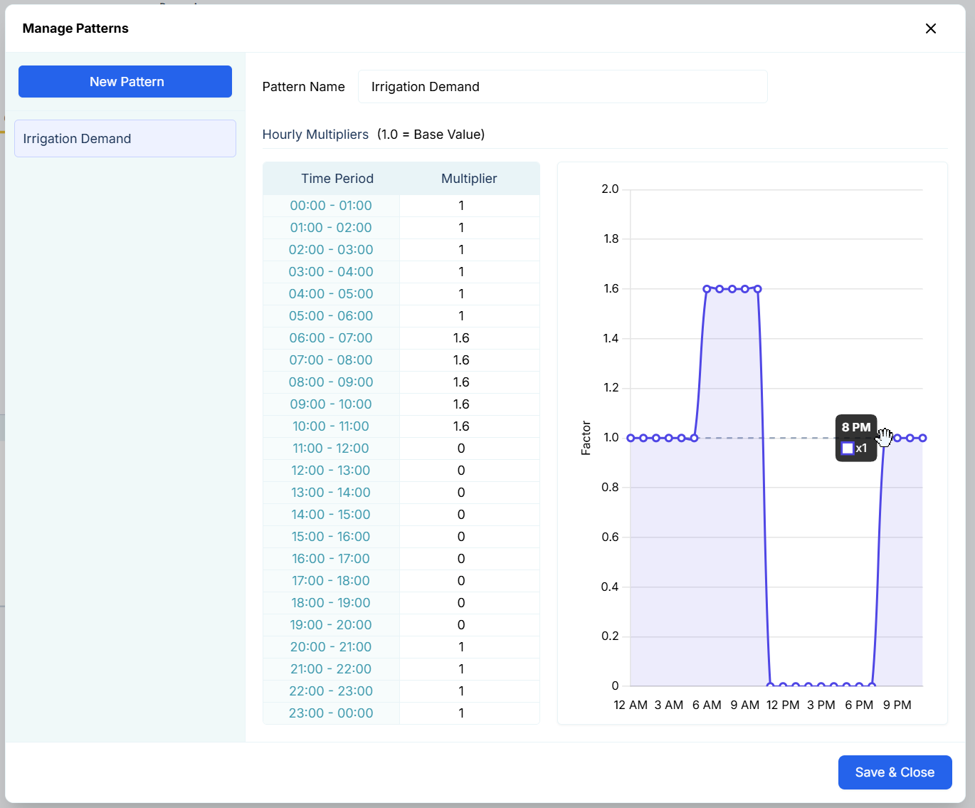
A pattern consists of 24 hourly multipliers representing a diurnal (daily) curve:
- A multiplier of 1.0 means the node draws exactly 100% of its Base Demand.
- A multiplier of 1.6 means the node draws 160% of its Base Demand during that hour.
- A multiplier of 0.0 means the flow is completely shut off.
You can edit these multipliers manually in the table on the left, or you can interactively click and drag the points on the graph on the right to shape your demand curve visually!
Stochastic Demand (Random Flow)
For advanced modeling, perfectly smooth demand curves aren't realistic. Real-world demand is "noisy" due to the random actions of individual consumers (flushing toilets, running dishwashers, turning on hoses). R-THYM can simulate this using the Enable Random Flow toggle.
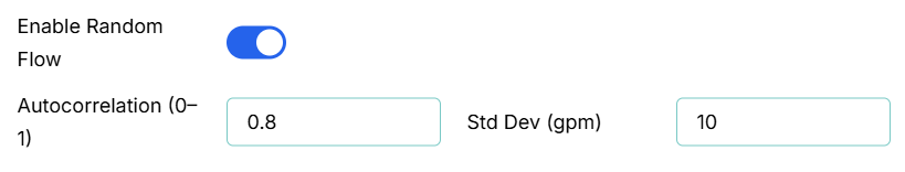
When enabled, the physics engine generates a continuous stochastic noise layer and overlays it on top of your Base Demand (and Pattern). You control the shape of this noise using two parameters:
- Std Dev (gpm): The Standard Deviation sets the amplitude or "spread" of the random fluctuations. A value of 10 means the flow will typically fluctuate within ±10 gpm of the target baseline.
- Autocorrelation (0–1): This controls the "memory" or smoothness of the random walk.
- A value near 0.0 produces high-frequency, choppy white noise (the flow bounces wildly every second).
- A value near 1.0 (e.g., 0.8 or 0.9) produces a smooth, wandering random walk (the flow gradually drifts up and down), which is highly representative of aggregated municipal demand.
Live Telemetry
Left-clicking an Outflow Node on the canvas during a simulation reveals its performance data in the right-hand Telemetry Panel.

The panel is split into the following sections:
- Instantaneous Metrics: Displays real-time values for the calculated Demand (the requested flow based on base demand and patterns) versus the actual Discharge leaving the node, alongside the Pressure (psi), Invert Elevation (ft), and the generation Mode (e.g., Random AR1).
- Hydraulic Chart: Dynamically plots the Discharge, Pressure, and Demand over time. In the screenshot above, you can clearly see the smooth, wandering stochastic noise applied to the flow rate because Random Flow was enabled!
- Active Warnings: If the local delivery pressure drops below the Min Pressure (psi) threshold defined in the properties, a red "Low pressure" warning will trigger at the bottom of the panel.